Fun With Diffusion Models | Cyprian Zander

Overview

In this project, I implemented generative models for image synthesis and denoising. In the first stage of the project, I worked with pretrained diffusion models, by using a DeepFloyd IF model with my own generated prompt embeddings. Using the pretrained model, I wrote sampling loops to produce images from noise, then extended the work to test out inpainting methods and optical illusions (like the visual anagram in this project’s cover picture). Later, I built generative models from scratch by training neural networks on MNIST. One of these models is a single-step denoising UNet trained to map noisy images to clean digits, which I then extended to a flow-matching model conditioned on noisy inputs and timesteps. I implemented the UNet architecture using down- and upsampling blocks with a loss objective to predict flow between noise and data distributions.

Part A: The Power of Diffusion Models

Part 0: Setup

To start out, I tested some prompt embeddings on the pretrained DeepFloyd model. The following text prompts were used to generate text embeddings:

a high quality picture
an oil painting of a snowy mountain village
a photo of the amalfi coast
a photo of a man
a photo of a hipster barista
a photo of a dog
an oil painting of people around a campfire
an oil painting of an old man
a lithograph of waterfalls
a lithograph of a skull
a man wearing a hat
a high quality photo
a rocket ship
a pencil
long-stemmed flowers strewn on the hood of a classic Porsche
a family of four sitting in a ski lift
a green tennis court

The last three prompts are my own.

I used a random seed (101) and upsampled the images from 64x64 to 256x256 using DeepFloyd’s pretrained stage II super-resolution model. For each of the below images, the output is the sampled output from 20, 50, and 100 steps from left to right.

Sampling Results

Prompt 1: a lithograph of waterfalls

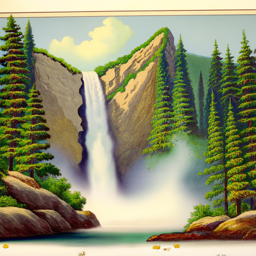
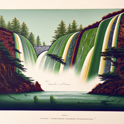
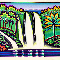
Across all of these images, the waterfalls are clearly recognizable, although adherence to the lithographic style is rather somewhat limited. Despite none of these samples reminding of true lithographies, the samples with higher step counts do seem to approach the idea of a drawing a more closely than the 20 step count image, which reminds more of an animated picture.

Prompt 2: long-stemmed flowers strewn on the hood of a classic Porsche

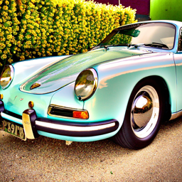
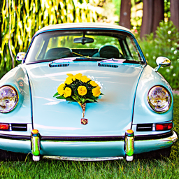
All of these renderings clearly display a Porsche, as indicated by the headlights and logo. However, the second iteration seemed to fail with the task of placing the flowers on the hood of the car and instead generated a flowery hedge behind the car. It seems that the 100 iteration image best adheres to the prompt, since it also incorporates the detail that the flowers are supposed to be long-stemmed. Curiously, all samples imagined a pale green vehicle, potentially hinting at some bias in the dataset regarding the green surroundings flowers are typically found in.

Prompt 3: a family of four sitting in a ski lift

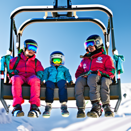
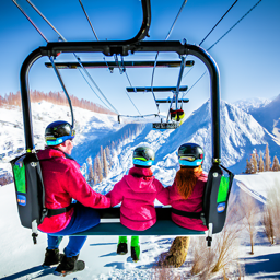
These images also closely adhere to the prompt provided, although only the 100 step example gets the number of people in the ski lift correct. Also notable is that all people were generated with helmets on, but none are correspondingly wearing skis or snowboards.

Prompt 4: a green tennis court

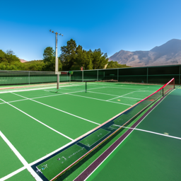
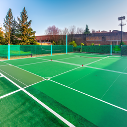
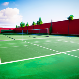
In this example, it seems that the model struggled with the combination of green coloring of a tennis court, presumably because tennis courts typically are not green, so the model had issues with correctly displaying the lines on a tennis court and the placement of the net.

Part 1: Sampling Loops

1.1: Implementing the Forward Process

In the first stage of implementing the diffusion model, I defined the forward diffusion process. The forward diffusion process gradually transforms a clean image $x_0$ into noise by scaling the signal and adding Gaussian noise. At timestep $t$, the image $x_t$ is sampled by

\[q(x_t \mid x_0) = \mathcal{N}\!\left(x_t;\ \sqrt{\bar{\alpha}_t}\, x_0,\ (1 - \bar{\alpha}_t)\mathbf{I}\right),\]

which is equivalent to

\[x_t = \sqrt{\bar{\alpha}_t}\, x_0 + \sqrt{1 - \bar{\alpha}_t}\, \varepsilon, \quad \varepsilon \sim \mathcal{N}(0, \mathbf{I}).\]

where $\bar{\alpha}_t$ is the cumulative product of the noise schedule up to timestep $t$. As $t$ increases, $\bar{\alpha}_t \to 0$, and $x_t$ becomes dominated by Gaussian noise.

You can see my code for my implementation of the forward(im, t).

Here is the Berkeley campanile at noise level [250, 500, 750].

$t=250, t=500, t=750$

1.2: Classical Denoising

To evaluate how difficult diffusion denoising is, I first applied a classical Gaussian blur to noisy images at timesteps $t \in {250, 500, 750}$. Gaussian filtering smooths high-frequency noise but cannot recover lost structure, so as the noise level increases, the images become increasingly blurred without meaningful reconstruction.

$t=250$

$t=500$

$t=750$

1.3: One-Step Denoising

In this step, I used stage_1.unet, a pretrained, timestep-conditioned UNet, to estimate the Gaussian noise present in a noisy image. Given a noisy image $x_t$, the timestep $t$, and a text prompt embedding, the UNet predicts the noise $\varepsilon$ that was added during the forward process, which I then appropriately scaled and removed to recover an estimate of the original image $x_0$.

Below is the original campanile, the noisy campanile at variable $t$ noise levels, and the corresponding one-step denoised campanile using the model.

$t=250$

$t=500$

$t=750$

As we can see, the denoising UNet is much better at projecting the image onto the natural image manifold, but the sharpness worsens with more noise.

1.4: Iterative Denoising

One-step denoising tries to recover a clean image $x_0$ directly from a noisy sample $x_t$, but diffusion models are designed to denoise gradually by repeatedly stepping from a noisier timestep to a less noisy one. Because running all $T=1000$ steps is expensive, I used a strided schedule and denoised only at those timesteps.

At each iteration we have an image $x_t$ at timestep $t=\texttt{strided_timesteps}[i]$, and we want to move to a less noisy timestep $t’=\texttt{strided_timesteps}[i+1]$. I first used the pretrained stage_1.unet (conditioned on $t$ and the text embedding) to estimate the noise $\hat{\varepsilon}$, then form an estimate of the clean image:

\[\hat{x}_0 \;=\; \frac{x_t - \sqrt{1-\bar{\alpha}_t}\,\hat{\varepsilon}}{\sqrt{\bar{\alpha}_t}}.\]

Then we update toward $t’$ using the iterative denoising rule, which is like linearly interpolating between signal and noise:

\[x_{t'} \;=\; \sqrt{\bar{\alpha}_{t'}}\,\hat{x}_0 \;+\; \sqrt{1-\bar{\alpha}_{t'}}\,\hat{\varepsilon} \;+\; \sigma(t,t')\,z,\]

where $z\sim \mathcal{N}(0,\mathbf{I})$. Repeating this update over the timesteps gradually projects the sample onto the natural image manifold, producing a much cleaner result than single-step denoising or Gaussian blur.

From left to right, iterative denoising at timesteps $690, 540, 390, 240, 90$

Original, iterative, one-step, original with Gaussian blur

1.5: Diffusion Model Sampling

Diffusion models can also be used as generative models by starting from pure Gaussian noise and iteratively denoising it. By setting i_start = 0 and initializing im_noisy with random noise, the iterative denoising process progressively removes noise according to the learned diffusion dynamics, guided by the text prompt embedding. This procedure transforms unstructured noise into a coherent image consistent with the prompt. In this example, I used the prompt embedding for “a high quality photo,” demonstrating how diffusion models generate images from scratch.

Five generated samples from the prompt 'a high quality photo'

1.6: Classifier-Free Guidance (CFG)

The unguided samples from the previous section look a bit nonsensical because, without strong conditioning, the denoising trajectory is only loosely constrained. Many different images are plausible under the model’s prior, and small errors in the predicted noise compound across iterative steps. With a weak prompt like the previous one (or effectively “null” conditioning), the model often drifts toward generic textures or unstable compositions instead of a coherent natural image.

Classifier-Free Guidance fixes this by explicitly steering the denoiser using both an unconditional and a conditional noise prediction. At each timestep I ran the UNet twice to get $\varepsilon_u$, a noise estimate with the unconditional prompt "" and $\varepsilon_c$, noise estimate with the conditional prompt embedding. Then, these can be combined using the CFG rule:

\[\varepsilon \;=\; \varepsilon_u + \gamma(\varepsilon_c - \varepsilon_u),\]

where $\gamma$ controls guidance strength. When $\gamma > 1$, the update amplifies the direction that moves the sample toward satisfying the text condition, producing more coherent images at the cost of reduced diversity. This guided $\varepsilon$ is then used in the same iterative denoising update as before.

Five samples with the prompt 'a high quality photo' and a CFG scale of $\gamma = 7$

1.7: Image-to-image Translation

Building on iterative denoising, we can extend diffusion beyond just generation by initializing the process from a real image instead of noise. SDEdit works by adding noise to a real input image and then running the diffusion denoising process to “project” it back onto the natural image manifold. The amount of noise controls edit strength: smaller i_start (less noise) preserves the original structure, while larger i_start (more noise) forces the model to hallucinate more missing information, producing larger, more creative changes. Using CFG from this point onward keeps the denoising trajectory stable and improves perceptual quality during this projection.

From left to right: Original, $i_{start}=1 (t=960)$, $i_{start}=3 (t=900)$, $i_{start}=5 (t=840)$, $i_{start}=7 (t=780)$, $i_{start}=10 (t=690)$, $i_{start}=20 (t=390)$

Here are some samples from my personal photo library.

From left to right: Original, $i_{start}=1 (t=960)$, $i_{start}=3 (t=900)$, $i_{start}=5 (t=840)$, $i_{start}=7 (t=780)$, $i_{start}=10 (t=690)$, $i_{start}=20 (t=390)$

1.7.1: Editing Hand-Drawn and Web Images

If SDEdit can project real photos back onto the image manifold, it should be even more effective when starting from inputs that lie far off that manifold. This same projection effect is even more dramatic for sketches or non-photorealistic web images. Starting from a drawing or stylized input, adding noise and denoising encourages the model to replace ambiguous strokes with fitting textures, lighting, and geometry, effectively “lifting” the input onto the natural image manifold. As i_start increases, the output becomes less faithful to the original lines and more like a realistic reinterpretation.

I decided to demonstrate this approach with an image downloaded from the web.

From left to right: Original, $i_{start}=1 (t=960)$, $i_{start}=3 (t=900)$, $i_{start}=5 (t=840)$, $i_{start}=7 (t=780)$, $i_{start}=10 (t=690)$, $i_{start}=20 (t=390)$

The same can be done for hand-drawn images. Here are two examples.

From left to right: Original, $i_{start}=1 (t=960)$, $i_{start}=3 (t=900)$, $i_{start}=5 (t=840)$, $i_{start}=7 (t=780)$, $i_{start}=10 (t=690)$, $i_{start}=20 (t=390)$

1.7.2: Inpainting

Inpainting uses the denoising loop while constraining part of the image to remain fixed. At every timestep, after producing a new sample, we overwrite the pixels outside the masked region with the original image content (with the correct noise level for that timestep), while leaving the masked region free to evolve. This forces the model to generate new content only inside the hole, while maintaining consistency with the unmasked context.

Below is the campanile inpainted with a different upper floor.

Original, mask, inpainted

1.7.3: Text-Conditional Image-to-image Translation

Text-conditional image-to-image translation is SDEdit plus language guidance. We start from a noised version of the input image, then denoise with CFG using a chosen prompt so the projection is biased toward satisfying the text. As i_start increases, the prompt influence becomes stronger because more of the final image must be hallucinated, producing outputs that both resemble the original image and increasingly reflect the text condition.

Here are three examples of the campanile and two of my own test images with the prompt ‘long-stemmed flowers strewn on the hood of a classic porsche’ applied.

From left to right: Original, $i_{start}=1 (t=960)$, $i_{start}=3 (t=900)$, $i_{start}=5 (t=840)$, $i_{start}=7 (t=780)$, $i_{start}=10 (t=690)$, $i_{start}=20 (t=390)$

1.8: Visual Anagrams

Once CFG-based sampling is stable, we can couple two different prompts by enforcing a symmetry constraint during denoising to create flip-dependent optical illusions.
At each timestep $t$, we predict noise in two “views” of the same latent: we run the UNet with prompt $p_1$ on $x_t$ to get $\varepsilon_1$, and we run the UNet with prompt $p_2$ on the flipped image $f(x_t)$ to get $\varepsilon_2$. We then flip $\varepsilon_2$ back and average the two noise estimates to form a single composite $\varepsilon$, and use that $\varepsilon$ in the reverse diffusion update; this forces the sample to satisfy $p_1$ in the upright orientation and $p_2$ when flipped.

You can see my corresponding code repository for my implementation of the visual_anagrams function. Below are two interesting illusions I created with this methodology.

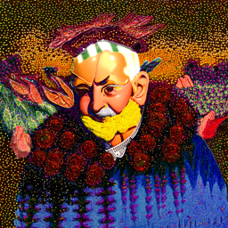
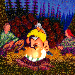
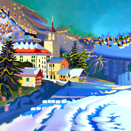
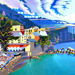
Prompts: 'An Oil Painting of an Old Man' and 'An Oil Painting of People around a Campfire'

1.9: Hybrid Images

Instead of coupling prompts by a geometric transform, we can couple them in the frequency domain by assigning one prompt to low frequencies and the other to high frequencies.
At each timestep $t$, I computed two CFG noise estimates from the same $x_t$: $\varepsilon_1 = \mathrm{CFG}(\mathrm{UNet}(x_t, t, p_1)),\qquad \varepsilon_2 = \mathrm{CFG}(\mathrm{UNet}(x_t, t, p_2)).$ We then combine them using the provided factorized rule: $\varepsilon \;=\; f_{\text{lowpass}}(\varepsilon_1)\;+\;f_{\text{highpass}}(\varepsilon_2),$ where $f_{\text{lowpass}}$ is a Gaussian blur (e.g., kernel 33, $\sigma=2$) and $f_{\text{highpass}}(x)=x-f_{\text{lowpass}}(x)$. Using this composite $\varepsilon$ in the denoising step makes the final image read as prompt $p_1$ at a distance (low-frequency structure) but reveal prompt $p_2$ up close (high-frequency detail).

You can see my corresponding code repository for my implementation of the visual_anagrams function. Below are two prompt combinations I created with this methodology.

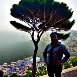
Prompts: "a photo of a man" and "a photo of the amalfi coast"

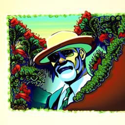
Prompts: "a lithograph of waterfalls" and "a man wearing a hat"

Part B: Flow Matching from Scratch

Before implementing and training the UNet, the goal is to rely on primary references for the core building blocks (convolutions, transposed convolutions, pooling, datasets, dataloaders, and training loops) so the architecture and optimization behavior are understood.

Part 1: Training a Single-Step Denoising UNet

1.1: Implementing the UNet

I implemented the denoiser as a UNet composed of downsampling and upsampling blocks with skip connections. The encoder progressively reduced spatial resolution while increasing channel depth to capture global context, and the decoder reconstructed the image while concatenating encoder features to preserve fine details. Operations such as convolutions, pooling, transposed convolutions, and channel-wise concatenation allowed the network to remain expressive without losing spatial information.

1.2: Using the UNet to Train a Denoiser

Once the architecture is defined, I trained it as a regression model that maps a noisy input back to a clean target with an L2 objective.
I generated training pairs $(x_{\text{noisy}}, x)$ on the fly by sampling a noise level $\sigma$ and forming $x_{\text{noisy}} = x + \sigma\varepsilon$ (with normalized $x$ and $\varepsilon \sim \mathcal{N}(0, I)$); the UNet $f_\theta$ is optimized to minimize $|f_\theta(x_{\text{noisy}}) - x|_2^2$, which encourages accurate pixel-level reconstruction.

Below is a visualization of the noising process.

From left to right: $\sigma \in \{0.0,\; 0.2,\; 0.4,\; 0.5,\; 0.6,\; 0.8,\; 1.0\}$

1.2.1: Training

I trained the denoiser on the MNIST training set for five epochs using shuffled batches. Noise was applied dynamically when each batch was fetched so that the model saw different corruptions of the same images across epochs, improving generalization. I used a UNet with hidden dimension $D=128$ and optimized it with Adam at a learning rate of $10^{-4}$, monitoring the training loss and visualizing denoised results on the test set after the first and fifth epochs.

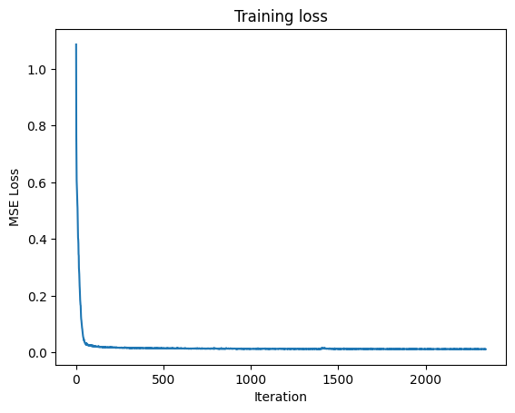
Training loss curve

After first epoch. Left: Original, Center: Noisy, Right: Denoised$

After fifth epoch. Left: Original, Center: Noisy, Right: Denoised$

1.2.2: Out-of-Distribution Testing

After training, I evaluated the denoiser on noise levels that were not seen during training. By keeping the same test images fixed and varying the noise magnitude, I observed how reconstruction quality degraded as the input distribution shifted. This experiment highlighted the limits of generalization for a denoiser trained on a restricted noise range.

Left: Noisy, $\sigma = 0.0, Right: Denoised$

Left: Noisy, $\sigma = 0.2, Right: Denoised$

Left: Noisy, $\sigma = 0.5, Right: Denoised$

Left: Noisy, $\sigma = 0.8, Right: Denoised$

Left: Noisy, $\sigma = 1.0, Right: Denoised$

1.2.3: Denoising Pure Noise

To explore denoising as a generative process, I trained the UNet to map pure Gaussian noise directly to clean-looking images. In this setup, the model learned to output the MSE-optimal prediction under extreme uncertainty. The resulting samples resembled blurred or averaged digit-like structures, reflecting the fact that minimizing MSE encourages predictions toward the mean of the training distribution rather than diverse, sharp samples.

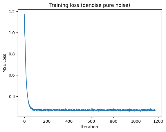
Training loss curve

Samples after first epoch

Samples after fifth epoch

A brief description of the patterns observed in the generated outputs and explanations for why they may exist.

Part 2: Training a Flow Matching Model

2.1: Adding Time Conditioning to UNet

After observing that one-step denoising and pure-noise denoising collapse to averaged prototypes, I needed a model that could explicitly represent how images evolve over multiple denoising steps.

I modified the UNet to be explicitly conditioned on the scalar timestep $t$ so the model could learn different behaviors at different noise levels. I implemented FCBlocks (small fully-connected networks built from nn.Linear) to embed a normalized $t \in [0,1]$, then used those embeddings to modulate intermediate decoder activations (e.g., scaling the unflatten and upsampling features) so the network could represent a time-dependent flow field rather than a single fixed denoising function.

2.2: Training the UNet

With time conditioning in place, training naturally shifted from predicting clean images to predicting how samples should move over time. I trained the time-conditioned UNet to predict the flow from an interpolated noisy sample $x_t$ back toward the clean image $x$ at a randomly sampled timestep $t$. For each batch, I sampled MNIST digits, sampled random $t$, constructed $x_t$ on-the-fly, and optimized the UNet with Adam (initial lr $=10^{-2}$) to regress the target flow, while using an exponential learning-rate decay scheduler stepped once per epoch. I tracked the training loss across the full run and plotted it as the primary training signal.

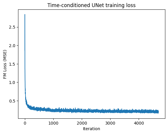
Training loss curve

2.3: Sampling from the UNet

Once the model learned a time-dependent flow field, I could use it to iteratively transform noise into data. I generated samples by starting from pure Gaussian noise and repeatedly applying the learned flow predictions across timesteps, gradually pushing samples toward the data manifold. I visualized outputs after 1, 5, and 10 epochs to show how training improved sample quality over time, with later checkpoints producing clearer and more structured digits.

2.4: Adding Class-Conditioning to UNet

While time conditioning enabled generation, it did not provide control over which digit was generated. I extended the UNet to accept a class-conditioning vector $c$ (a one-hot encoding for digits 0–9) by adding additional FCBlocks and combining class and time embeddings to modulate decoder activations. To retain unconditional generation capability, I applied conditioning dropout by zeroing the class vector 10% of the time, enabling classifier-free guidance during sampling.

2.5: Training the UNet

With both time and class conditioning integrated, training followed the same flow-matching objective with additional supervision. I trained the class-conditioned UNet using the same procedure as the time-only model, except that each batch included a class vector that was randomly dropped with fixed probability. I recorded and plotted the training loss across epochs to analyze convergence and stability relative to the time-only model.

2.6: Sampling from the UNet

Finally, I combined class conditioning with classifier-free guidance to improve both fidelity and controllability during generation. I sampled images by specifying a target digit class and applying classifier-free guidance during iterative denoising, generating results after 1, 5, and 10 epochs (four samples per digit). I also experimented with removing the exponential learning-rate scheduler and compensated through alternative optimization choices, comparing the resulting visual quality to the scheduled baseline.