Neural Radiance Fields

Overview

In this project, I built a pipeline for rendering Neural Radiance Fields from images. First, I calibrated my camera using ArUco markers, estimated poses for a 30–50 images of an object, and combined the intrinsics, poses, and undistorted images into a dataset. I then implemented a NeRF by generating camera rays, sampled points along each ray, encoded them with positional encodings, and used an MLP to predict colors and densities. Finally, I used volume rendering to synthesize new views of the object.

Part 0: Calibrating Your Camera and Capturing a 3D Scan

0.1: Calibrating Your Camera

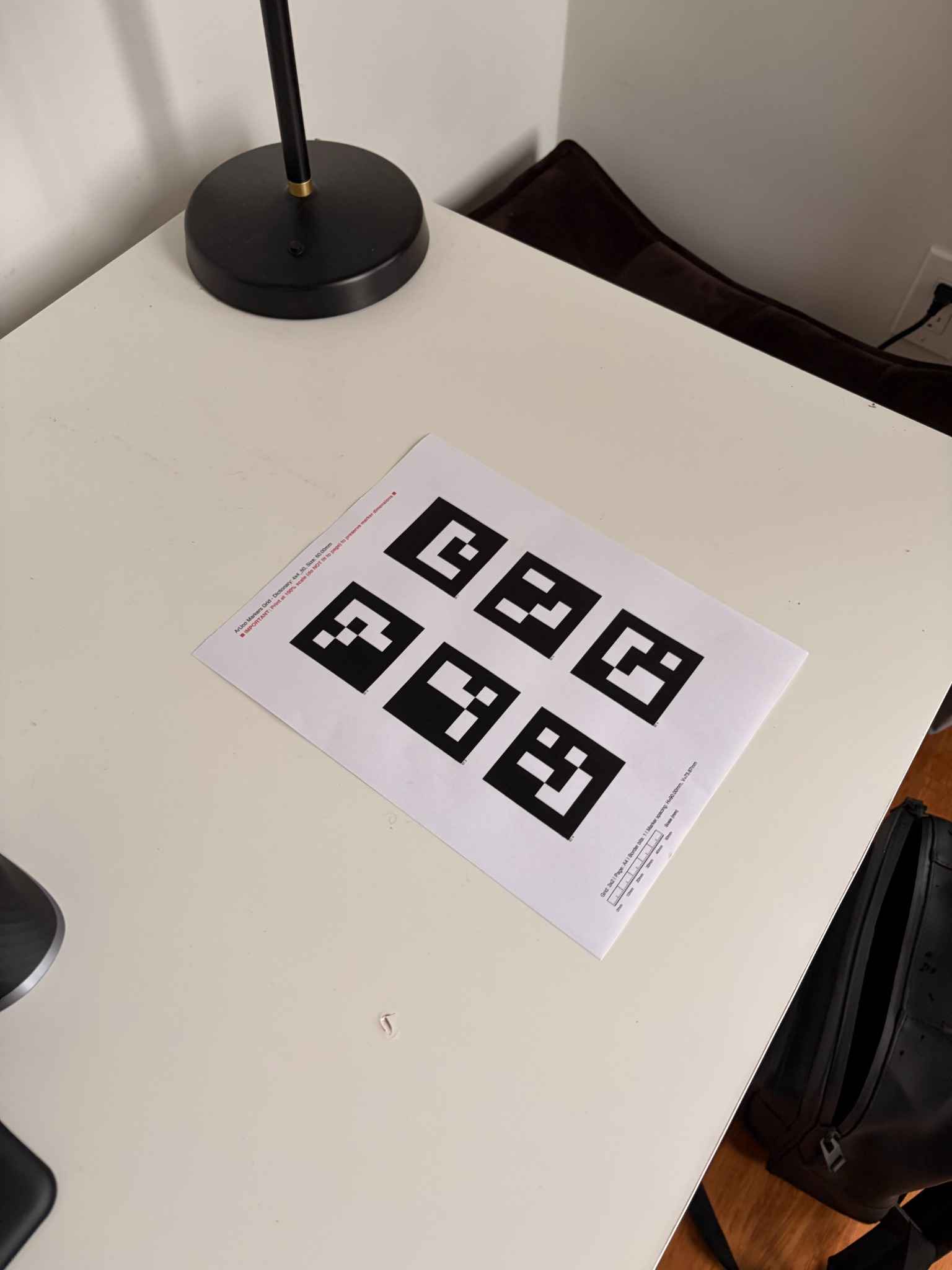
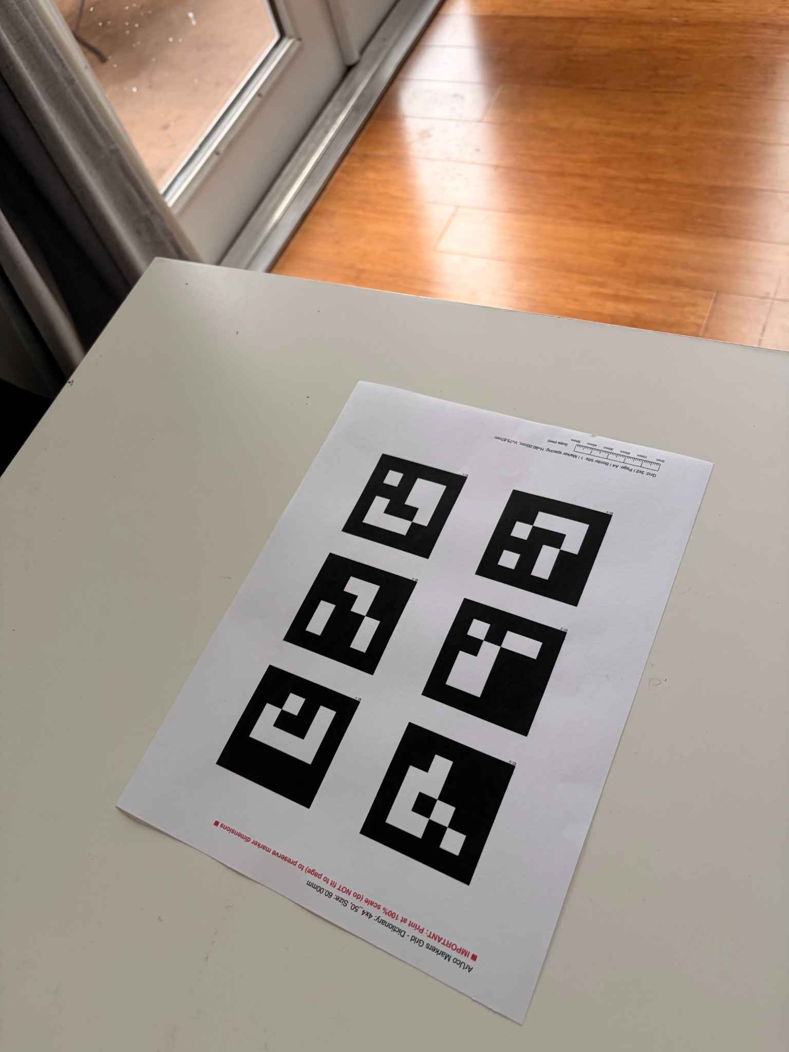
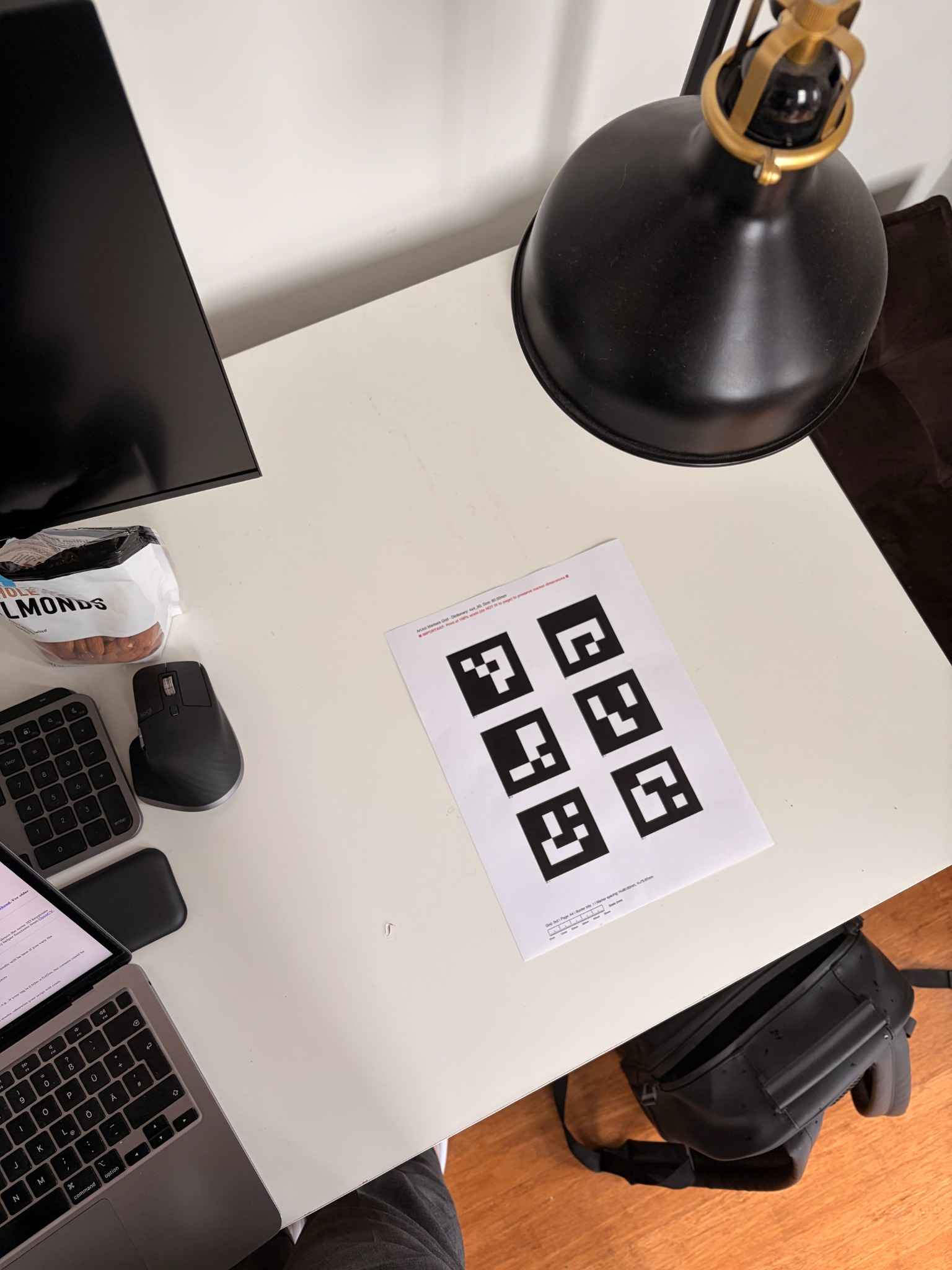
I calibrated my camera using ArUco markers, capturing 37 images from different angles. For each image, I collected the marker’s 4x4 corner. The calibrateCamera function in OpenCV helped compute the camera intrinsics and distortion coefficients, which would be useful for my own object dataset curation later.

Below are some sample images.

0.2: Capturing a 3D Object Scan

For my target NeRF reconstruction, I captured around 35 images of a LEGO model from different angles at a consistent distance, keeping the same camera and zoom level as the calibration dataset.

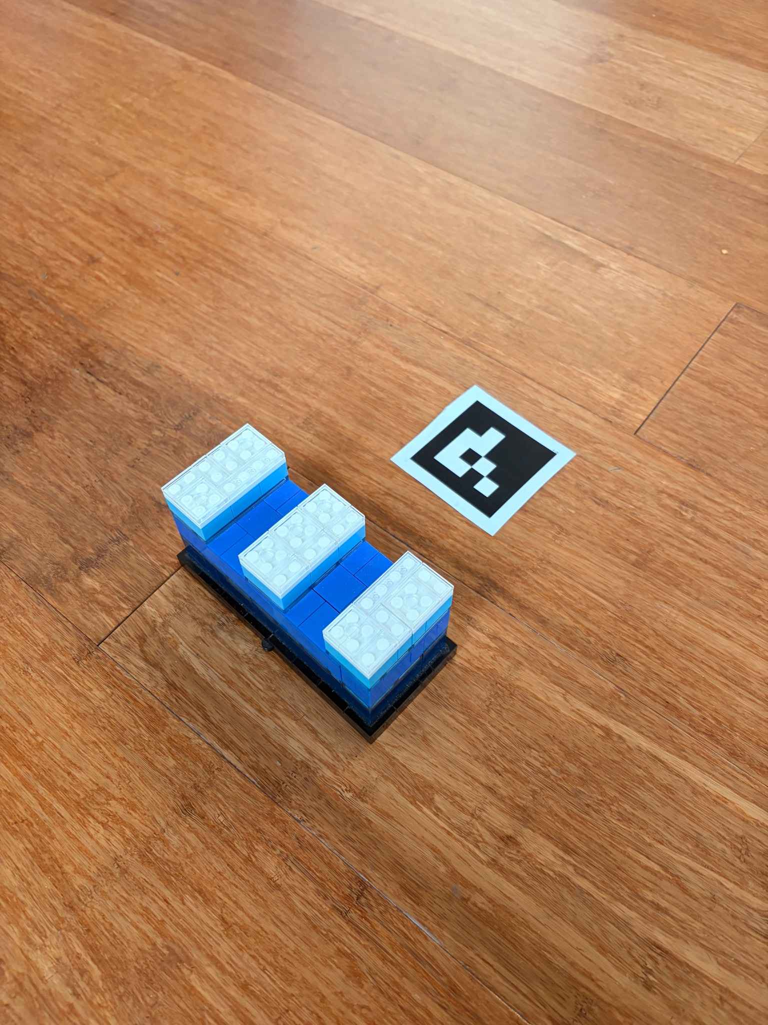
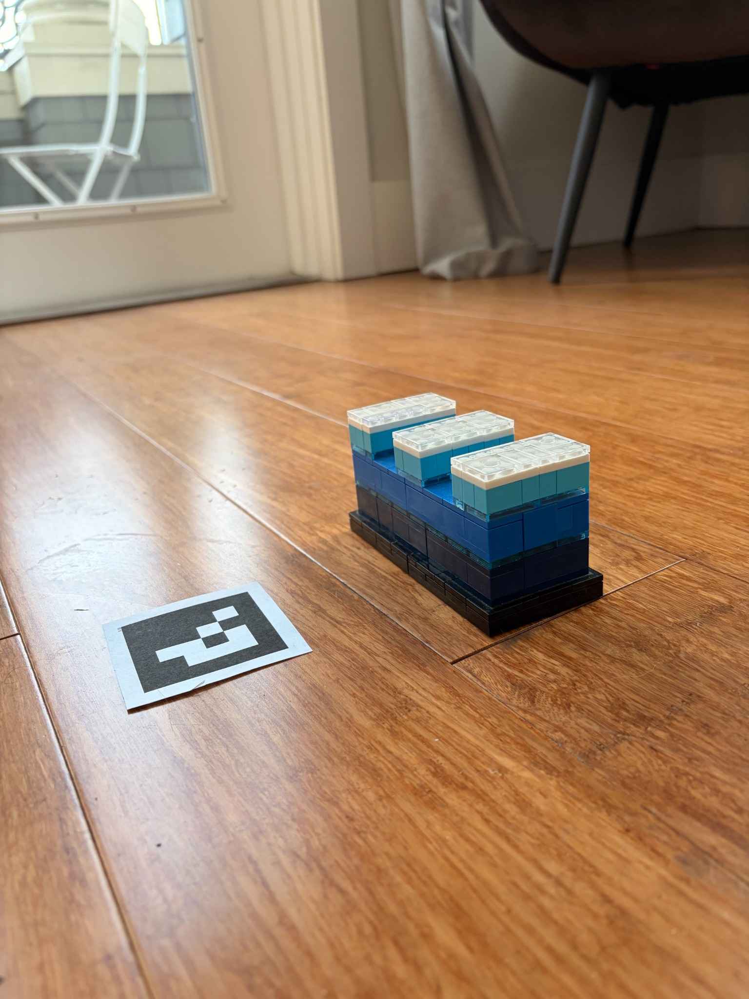
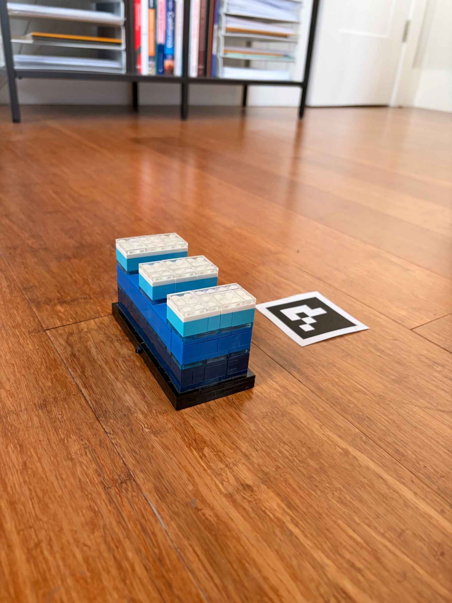
0.3: Estimating Camera Pose

For each image containing the ArUco marker, I solved the Perspective-n-Point (PnP) to estimate the camera pose by matching the detected 2D corner positions with their known 3D coordinates. This returns a rotation vector and translation vector representing transformation between the world and the camera. With the viser library, I visualized all of the poses for each image in the dataset.

0.4: Undistorting images and creating a dataset

In the final step of the data preparation process, I removed the lens distortion from each image to make sure they match the pinhole camera model that NeRF assumes. To eliminate black borders from undistortion, I computed an undistored camera matrix, cropped the images to the valid ROI, and adjusted the principal point coordinates to account for the crop offset. Finally, I split the undistorted images and their c2w poses into training, validation, and test sets.

Part 1: Fit a Neural Field to a 2D Image

Before working with 3D Neural Radiance Fields, I first implemented a 2D neural field. For this, I built an MLP that takes normalized 2D pixel coordinates as input and outputs RGB color values. To capture high-frequency details, I applied sinusoidal positional encoding to the input coordinates, expanding them from 2D to higher dimensions: $\gamma(p) = [p, \sin(2^0\pi p), \cos(2^0\pi p), \ldots, \sin(2^{L-1}\pi p), \cos(2^{L-1}\pi p)]$ where $L$ is the maximum frequency level. The network was trained using MSE loss between predicted and ground truth colors, optimized with Adam and evaluated using the Peak Signal to Noise Ratio (PSNR).

The neural field consists of a 4-layer MLP of variable width (I tested 64 and 256 channels), ReLU activations between layers, and a final Sigmoid activation. I trained for 1000 iterations with a batch size of 10,000 randomly sampled pixels per iteration, using Adam optimizer with learning rate $0.01$.

Here you can see some examples of the neural field inference across increasing iterations.

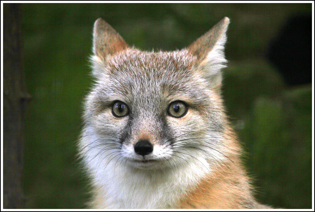
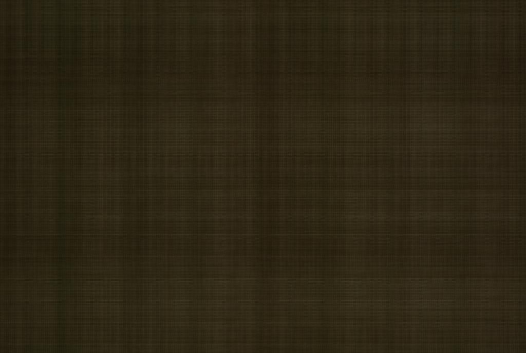
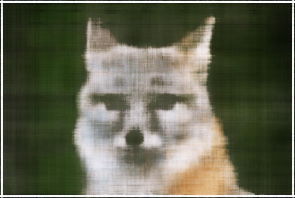
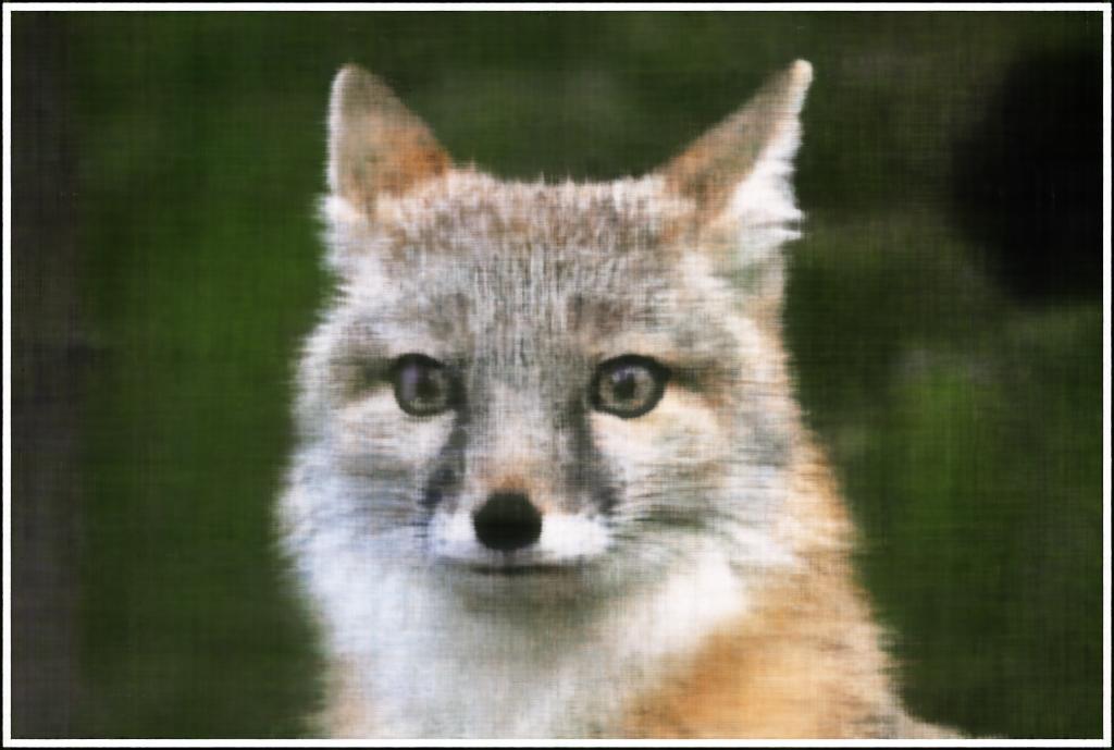
Original, 0 iterations, 100 iterations, 900 iterations.

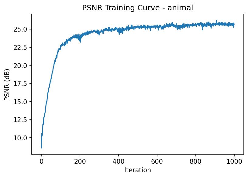
Below is a grid displaying fully trained results from tweaking positional encoding frequencies and network widths.

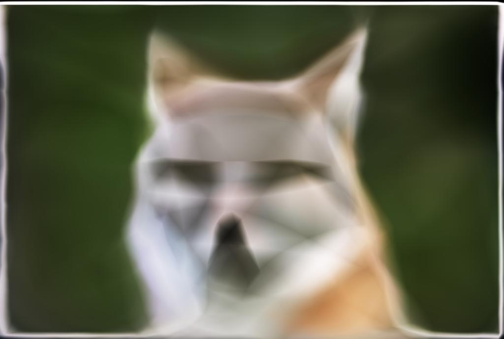
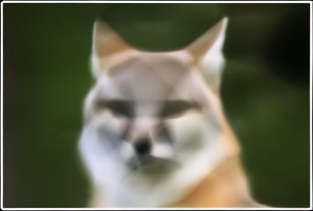
max_freq=2; left, width=64, right width=256

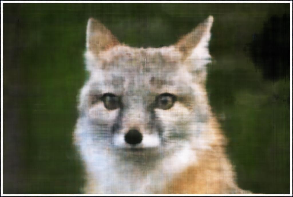
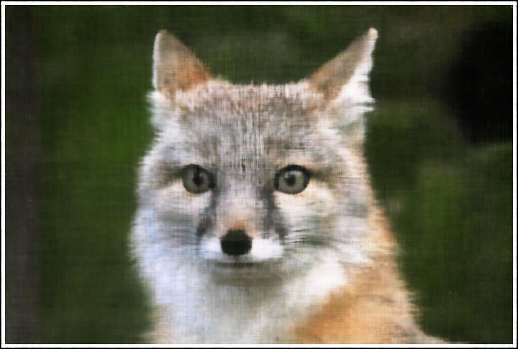
max_freq=10; left, width=64, right width=256

With a low frequency encoding, the reconstruction loses high-frequency details and appears blurry. With narrow linear layers (width=64), the model struggles to capture fine details even with high-frequency encoding. The best results come from max_freq=10 with width=256, achieving a sharp reconstruction of the original image.

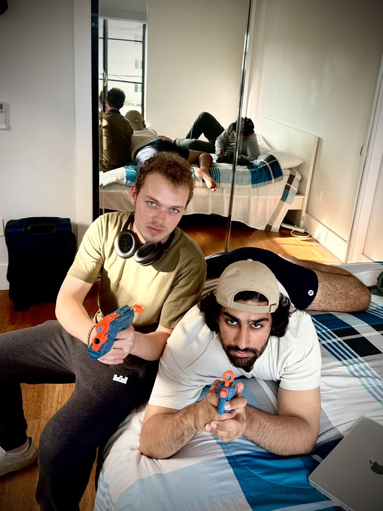
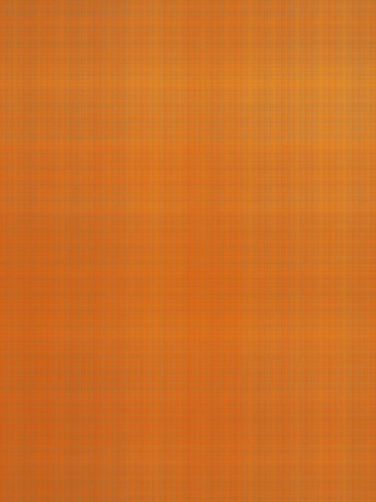
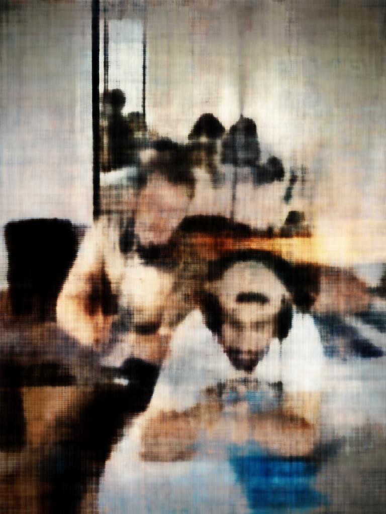
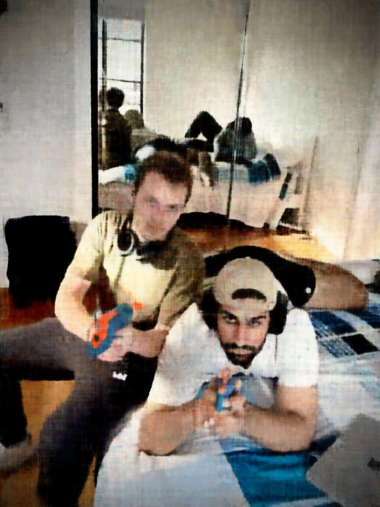
Original, 0 iterations, 100 iterations, 900 iterations. It's NeRF or Nothing.

Part 2: Fit a Neural Radiance Field from Multi-view Images

2.1: Create Rays from Cameras

Moving into 3D space, to render novel views with NeRF, I first needed to generate camera rays for each pixel. I implemented three transformation functions to convert pixel coordinates into 3D rays in world space.

First, I implemented transform(c2w, x_c) to convert points from camera coordinates to world coordinates using the camera-to-world matrix from part 0.1. Given a transformation defined by rotation $R$ and translation $t$, this applies $\mathbf{x}_w = R \mathbf{x}_c + t$.

Next, I implemented pixel_to_camera(K, uv, s) to convert pixel coordinates back to camera space. Given the intrinsic matrix:

and the projection equation $s \mathbf{u} = K \mathbf{x}_c$, I inverted this to get:

Finally, I combined these in pixel_to_ray(K, c2w, uv) to generate rays. For each pixel, the ray origin is simply the camera position $\mathbf{o} = c2w[:3, 3]$. To find the ray direction, I computed a point at depth $s=1$ in camera space, transformed it to world space, and normalized the direction: $\mathbf{d} = \frac{\mathbf{x}_w - \mathbf{o}}{|\mathbf{x}_w - \mathbf{o}|}$.

2.2: Sampling

For training, I had to sample rays from multiple images and discretize each ray into 3D sample points. I implemented sample_rays(images, Ks, c2ws, N) to select $N$ rays from all pixels across all images. I created a pixel grid for all images, added 0.5 to convert from image coordinates to pixel centers, then globally sampled ray indices. For each sampled ray, I computed its origin and direction using the corresponding camera’s intrinsics and extrinsics, along with the ground truth pixel color.

To sample points along each ray, I implemented sample_points_along_rays(origins, directions, near, far, n_samples) which discretizes rays between near and far planes (set to 2.0 and 6.0 for the lego scene). Rather than using uniform samples $t = \text{linspace}(\text{near}, \text{far}, n)$ which may cause overfitting, I introduced stratified sampling with perturbations during training. I divided the ray into equal intervals, then randomly sampled within each interval to ensure every location along the ray gets visited during training. The final 3D coordinates are computed as $\mathbf{p} = \mathbf{o} + t \mathbf{d}$ for each sample distance $t$.

2.3: Putting the Dataloading All Together

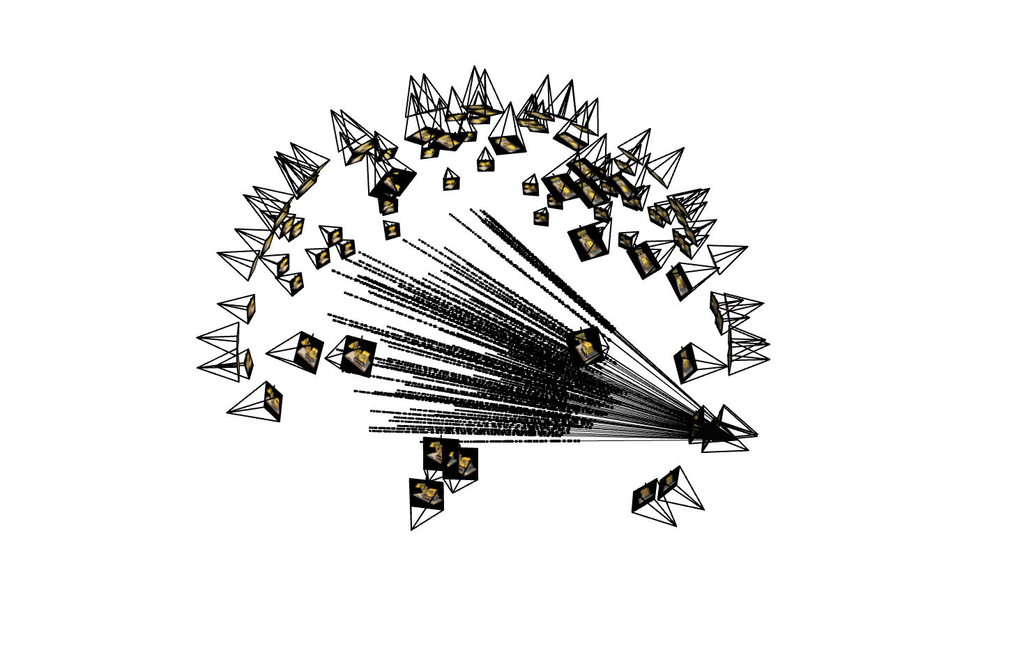
Finally, I combined the ray generation and sampling functions into a RaysData class that precomputes all rays for the training images. The dataloader stores pixel coordinates, calculates ray origins and directions for every pixel across all images, and maps them to their corresponding ground truth colors. During training, the sample_rays(N) method randomly selects $N$ rays along with their colors for each batch. I verified the implementation using viser to visualize the camera frustums, sampled rays, and 3D sample points, confirming that rays correctly travel from camera positions and sample points lie along the expected ray paths.

Below is the viser visualization for an initial Lego wheel loader dataset.

2.4: Neural Radiance Field

With the data preparation ready, I implemented the NeRF MLP to predict RGB color and volume density for 3D points. As an extension to the 2D neural field, this network takes both the 3D world coordinates and viewing directions as inputs, since color in a radiance field intuitively depends on view angle. I applied positional encoding to both inputs, using higher frequency for positions ($L=10$) to capture fine geometric details and a lower frequency for directions ($L=4$), which ensured that viewing-dependent effects would be smoother.

In this extended model, the architecture consists of eight fully connected layers with ReLU activations. After the first 4 layers, I concatenated the original positionally-encoded coordinates back into the network as a skip connection, which helps retain spatial information. The network then splits into two components. First, there’s a density head that outputs a single positive value (using ReLU), and a color head that takes the intermediate features concatenated with the encoded viewing direction to produce RGB values (with Sigmoid activations to bound outputs to [0,1]).

For my own dataset’s model, I scaled the layers to 512.

2.5: Volume Rendering

With the NeRF network predicting colors and densities at sampled 3D points, I implemented volume rendering to composite these samples into final pixel colors. The continuous volume rendering equation is:

where $T(t) = \exp\left(-\int_{t_n}^{t} \sigma(\mathbf{r}(s)) \, ds\right)$ is the probability of a ray reaching point $t$ without hitting anything. For discrete samples, this becomes:

where $\alpha_i = 1 - \exp(-\sigma_i \delta_i)$ is the probability of the ray terminating at sample $i$ with step size $\delta_i$, and $T_i = \prod_{j=1}^{i-1}(1 - \alpha_j)$ is the accumulated transmittance. I implemented this using torch.cumprod to compute the transmittance efficiently, allowing gradients to flow back through the rendering process during training.

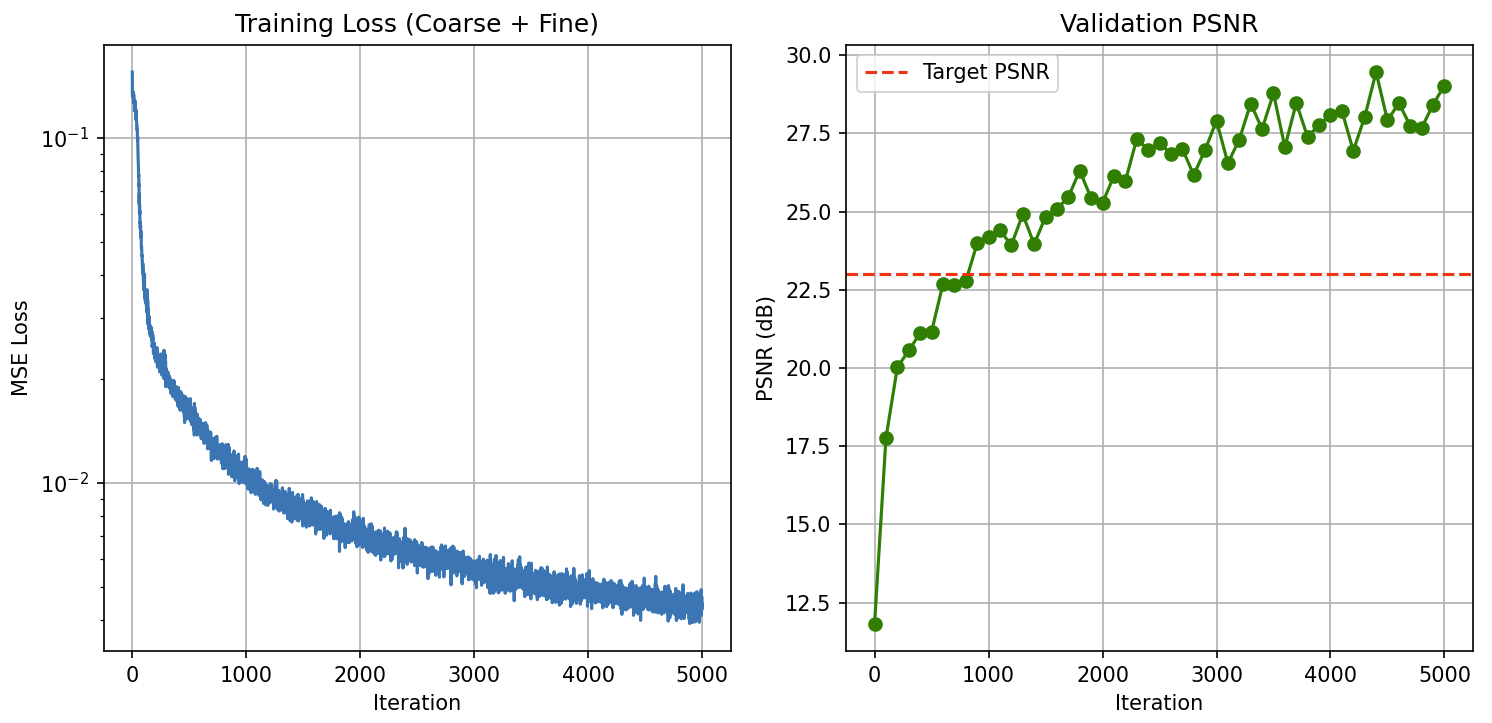
I trained the NeRF using Adam optimizer with learning rate $0.0005$, sampling 10,000 rays per batch for 5000 iterations. The model was optimized using MSE loss between rendered and ground truth colors, reaching over 23 PSNR on the validation set.

Below is the novel view synthesis on the wheel loader dataset.

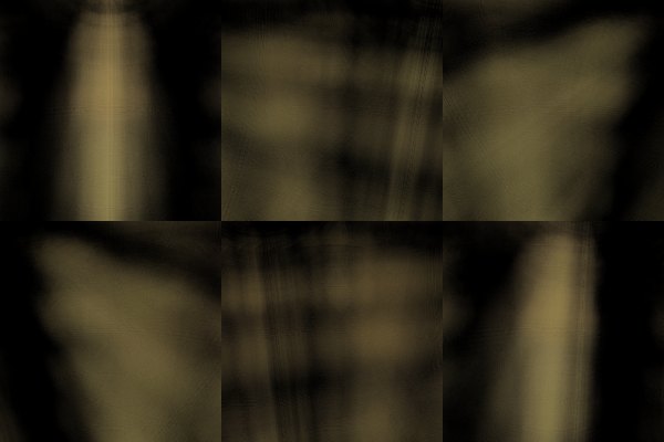
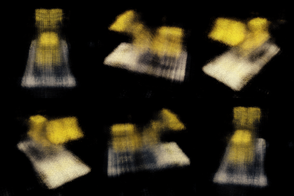
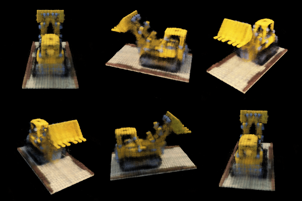
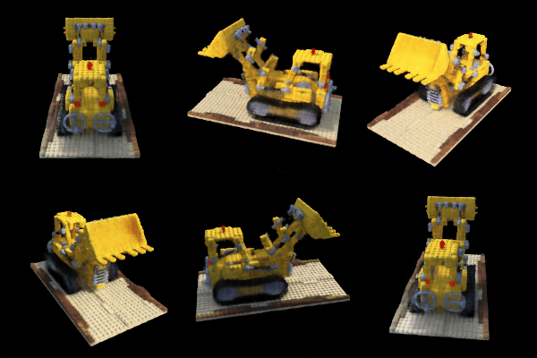
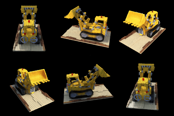
iterations: 100, 300, 1000, 3000, 5000.

2.6: Training with your own data

For my own dataset, I trained a NeRF on the LEGO dataset collected earlier. To accommodate the real-world capture conditions, I adjusted several hyperparameters from the synthetic lego dataset. Most importantly, I tuned the near and far sampling bounds to 0.02 and 0.5 based on the actual distance between my camera and the object. I also increased the number of samples per ray from 32 to 64 for higher quality reconstruction, which increased training time but significantly improved detail.

To generate novel views, I implemented a circular camera trajectory that orbits around the object while maintaining focus on the scene center using a look_at_origin function. I generated 60 frames by rotating the camera position around the object and rendering each view through the trained NeRF. The training process showed steady improvement in reconstruction quality, with the PSNR increasing as the network learned to represent the 3D structure and appearance.

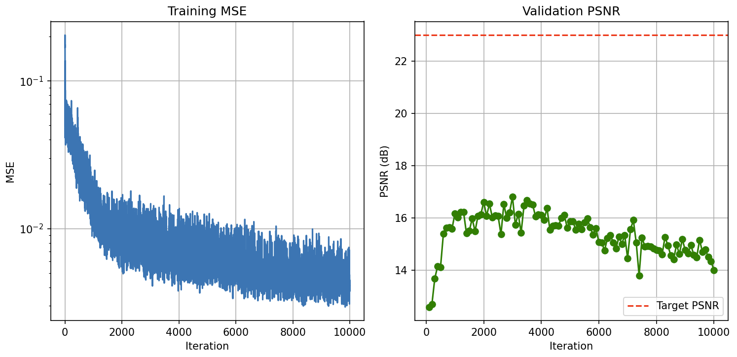
Below is the novel view synthesis on the wheel loader dataset.

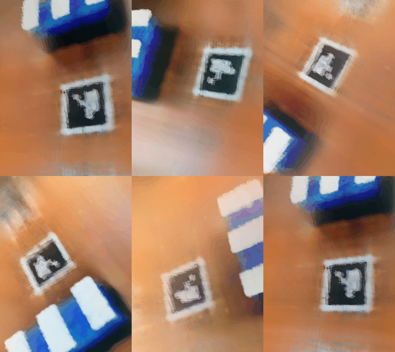
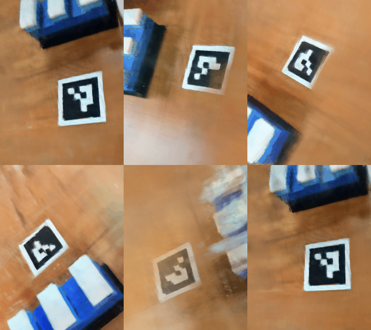
iterations: 1000, 5000, 10000.

Bonus: Another NeRF render!