Fun with Filters and Frequencies
September 26, 2025
Overview
In this project, I explored edge detection with finite differences and Gaussian smoothing, image sharpening with unsharp masking, hybrid images by mixing high and low frequencies, and multi-resolution blending with Gaussian and Laplacian stacks for seamless composites.
Part 1: Fun with Filters
1.1 Convolutions from Scratch
Convolutions are mathematical operations applied to images to extract features, such as edges. In this context, a kernel (or filter) slides across the image, performing element-wise multiplication and summation with the overlapping region at each position.
I implemented two convolution methods from scratch in NumPy:
-
convolve2d_np_four: For each pixel, the kernel is flipped and multiplied with the corresponding image patch using four nested loops, directly computing the convolution sum. -
convolve2d_np_two: This method improves efficiency by extracting a region from the padded image and computing the convolution sum with the flipped kernel using only two loops.
def convolve2d_np_four(i, k):
    h, w = i.shape
    kh, kw = k.shape

    i_pad = np.pad(i, ((kh // 2, kh // 2), (kw // 2, kw // 2)), mode='constant', constant_values=0)

    k_flip = np.flip(k)

    out = np.zeros((h, w))
    for i in range(h):
        for j in range(w):
            for ki in range(kh):
                for kj in range(kw):
                    out[i, j] += i_pad[i + ki, j + kj] * k_flip[ki, kj]

    return out

def convolve2d_np_two(i, k):
    h, w = i.shape
    kh, kw = k.shape

    i_pad = np.pad(i, ((kh // 2, kh // 2), (kw // 2, kw // 2)), mode='constant', constant_values=0)

    k_flip = np.flip(k)

    out = np.zeros((h, w))
    for i in range(h):
        for j in range(w):
            roi = i_pad[i:i+kh, j:j+kw] # full pixel-wise convolution
            out[i, j] = np.sum(roi * k_flip)

    return out
For clarity, padding is applied to the image to ensure that the convolution operation can be performed at the edges. Adding a border of zeros around the image allows the algorithm to apply the convolution at every pixel in the image. Flipping the kernel is necessary to perform convolution, rather than cross-correlation.
Filters
Below are three sample kernels I used to convolve some images.
This finite difference filter detects vertical edges by computing the difference between horizontal pixel intensities.
$$ D_x = \begin{bmatrix} 1 & 0 & -1 \end{bmatrix} $$This finite difference filter detects horizontal edges by computing the difference between vertical pixel intensities.
$$ D_y = \begin{bmatrix} 1 \\ 0 \\ -1 \end{bmatrix} $$This filter replaces each pixel with the average of its neighbors (blur).
$$ Box = \frac{1}{81} \begin{bmatrix} 1 & 1 & 1 & 1 & 1 & 1 & 1 & 1 & 1 \\ 1 & 1 & 1 & 1 & 1 & 1 & 1 & 1 & 1 \\ 1 & 1 & 1 & 1 & 1 & 1 & 1 & 1 & 1 \\ 1 & 1 & 1 & 1 & 1 & 1 & 1 & 1 & 1 \\ 1 & 1 & 1 & 1 & 1 & 1 & 1 & 1 & 1 \\ 1 & 1 & 1 & 1 & 1 & 1 & 1 & 1 & 1 \\ 1 & 1 & 1 & 1 & 1 & 1 & 1 & 1 & 1 \\ 1 & 1 & 1 & 1 & 1 & 1 & 1 & 1 & 1 \\ 1 & 1 & 1 & 1 & 1 & 1 & 1 & 1 & 1 \end{bmatrix} $$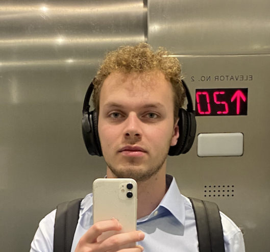
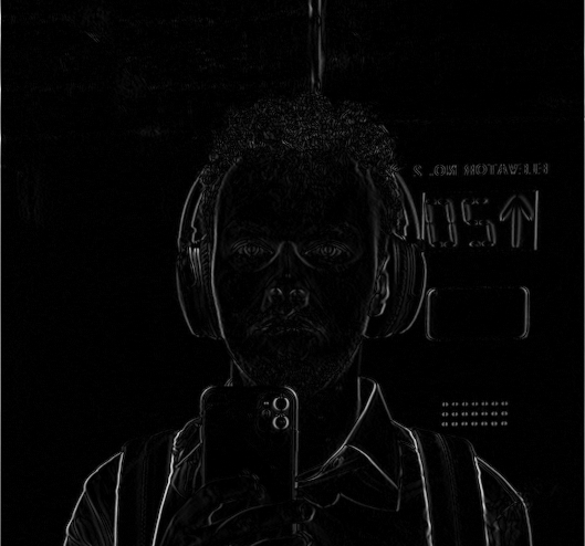
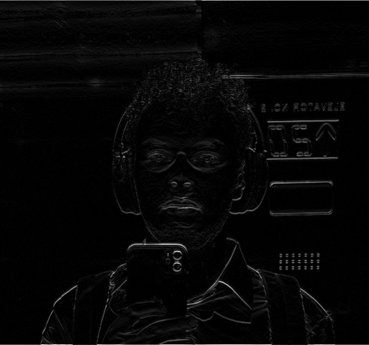
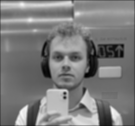
From left to right, the original, $D_x$ applied to it, then $D_y$, then the box filter.
Efficiency and Accuracy of Convolution Implementations
Here is a summary of the compute time I observed when performing the 9x9 box filter convolution on the above image, compared to scipy.signal.convolve2d as a benchmark, along with a comparison of differences to the output provided by the SciPy method.
| Implementation | Time Taken (s) | Max Difference to SciPy |
|---|---|---|
| Four loops | 10.100 | 1.44e-15 |
| Two loops | 0.956 | 5.55e-16 |
| SciPy | 0.041 | 0 |
As can be seen, the maximum differences from the reference function are extremely small, which can be attributed to minor variations in floating-point precision.
1.2 Finite Difference Operator
I used finite difference operators to compute the derivative of an image, highlighting regions with large intensity changes (what our eyes perceive as edges). By calculating the gradient magnitude from the \(D_x\) and \(D_y\) filters (by simply computing the magnitude of both filtered images combined), I produced a composite edge-detection image.
For example, I first applied the \(D_x\) and \(D_y\) filters to the reference image shown on the left.
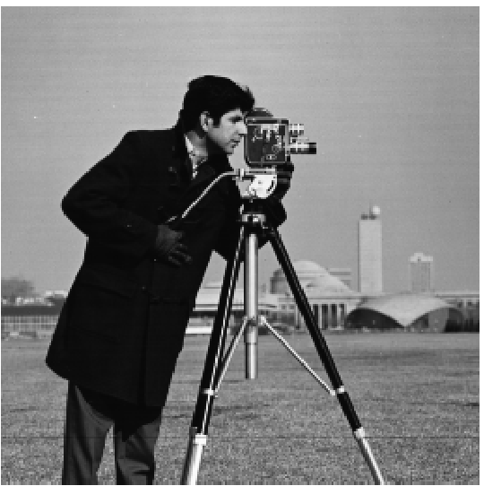
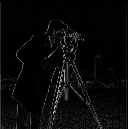
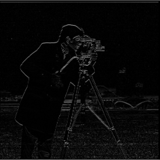
Left: Original, Center: $D_x$, Right: $D_y$.
Next, I computed the gradient magnitude between the two convolutions, as seen in the first image below, and manually set a threshold to isolate edges from noise.
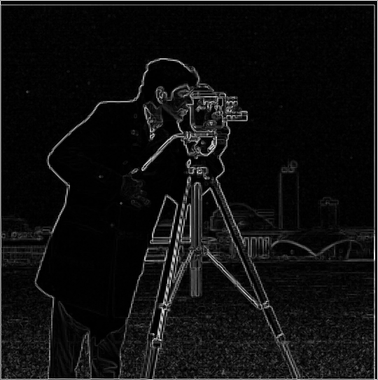

Left: Gradient magnitude image, Right: Binarized edge image.
I selected a pixel intensity threshold of 0.3 to classify edges. My reasoning was that I preferred to preserve edge continuity, even if it meant retaining some noise in the image. This threshold struck a healthy balance, eliminating most of the noise in the grass while almost perfectly maintaining the outline of the subject.
Nevertheless, these edge detections still appear somewhat noisy, so in the next section I explore the use of Gaussian blurs to clean up the output.
1.3 Derivative of Gaussian (DoG) Filter
To smooth our binarized edge image, I first applied a 2D Gaussian filter (outer product of a 1D Gaussian) to the original image before applying the \(D_x\) and \(D_y\) filters. Applying a Gaussian filter reduces high-frequency noise in the image, which helps the finite difference filters produce cleaner and more continuous edge detections. Below is each step in the procedure.


Left: Original, Right: Gaussian blur applied ($kernel~size = 15$, $\sigma=2$).


Left: $D_x$ filter applied on blurred image, Right: $D_y$ filter applied on blurred image.


Left: Gradient magnitude composite, Right: Binarized edge image.
The order of convolutions can also be changed, by first convolving the Gaussian blur with the finite difference filters to produce a Derivative of Gaussian filter (DoG). This works because convolution is a linear and shift-invariant operation, so the order of convolution can be rearranged. In other words, \((G * D_x) * I = G * (D_x * I)\), where $G$ is the Gaussian filter and $I$ is the image.


Left: $D_x$ DoG, Right: $D_y$ DoG.
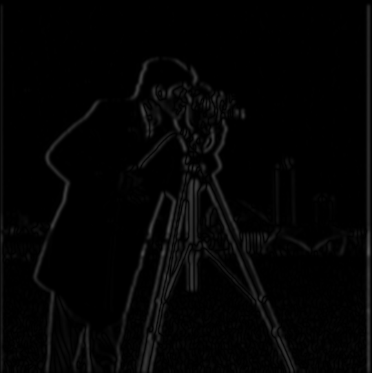
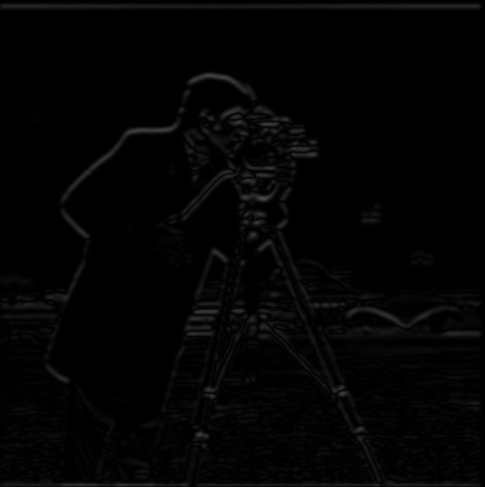
Left: Original convolved on $D_x$ DoG, Right: Original convolved on $D_y$ DoG.
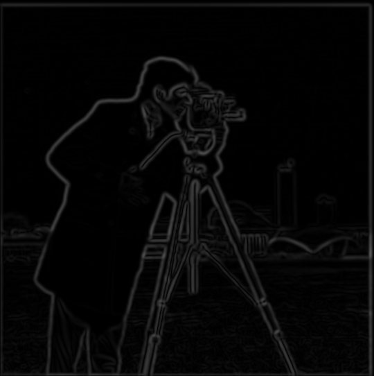
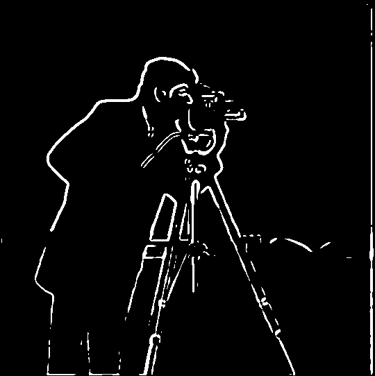
Left: Gradient magnitude composite, Right: Binarized edge image.
| Comparison | Max Difference |
|---|---|
| dx (DoG vs. Blurred) | 1.30e-15 |
| dy (DoG vs. Blurred) | 1.35e-15 |
As before, the maximum differences between the DoG and blurred approaches are extremely small, which is simply variation in floating-point precision, confirming that the order of operations yields identical results.
Part 2: Fun with Frequencies
2.1 Image Sharpening (Unsharp Mask)
Next, I implemented an image sharpening technique, by creating an unsharp mask filter. It works by first blurring the original with a Gaussian filter, which is then subtracted from the original, isolating the high-frequency components. By adding more of these high frequencies scaled by some strength paramater into the original image, the unsharp mask filter pronounces edges, producing a ‘sharpening’ effect. Below are some examples.


Left: High frequencies, Center: Original Taj Mahal Right: Sharpened Taj Mahal ($factor=1.2$).
Some more examples from my personal photo library:
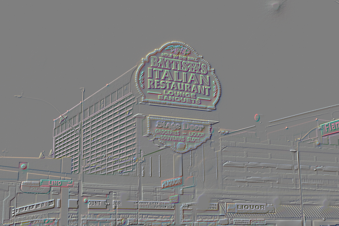


Left: High frequencies, Center: Original Las Vegas sign Right: Sharpened Las Vegas sign ($factor=1.2$).
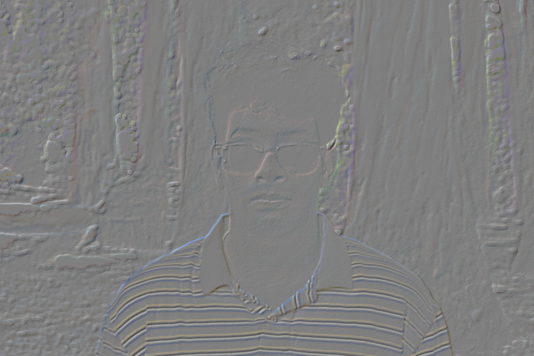
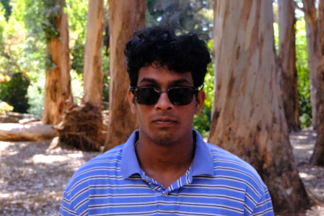
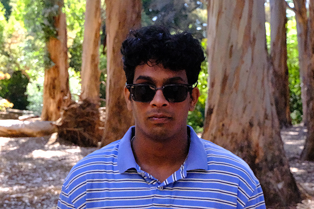
Left: High frequencies, Center: Original Shenoy, Right: Sharpened Shenoy ($factor=3$).
Note: The last image is sharpened using a higher strength factor than the previous examples. While this increases the prominence of edges, it also amplifies high-frequency noise present in the image, producing a grainier appearance. This demonstrates that too much sharpening can enhance unwanted details and artifacts. For a final demonstration of the sharpening process, I intentionally blurred an image, then applied the unsharp mask to assess how well the original can be reconstructed. Results are below:

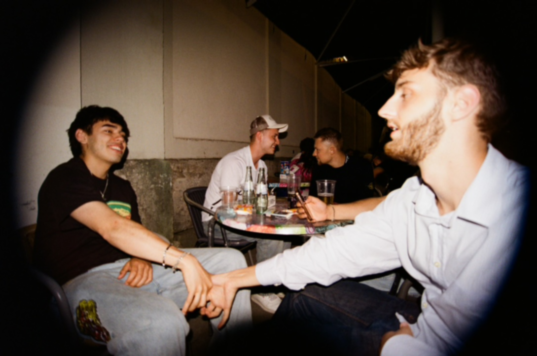
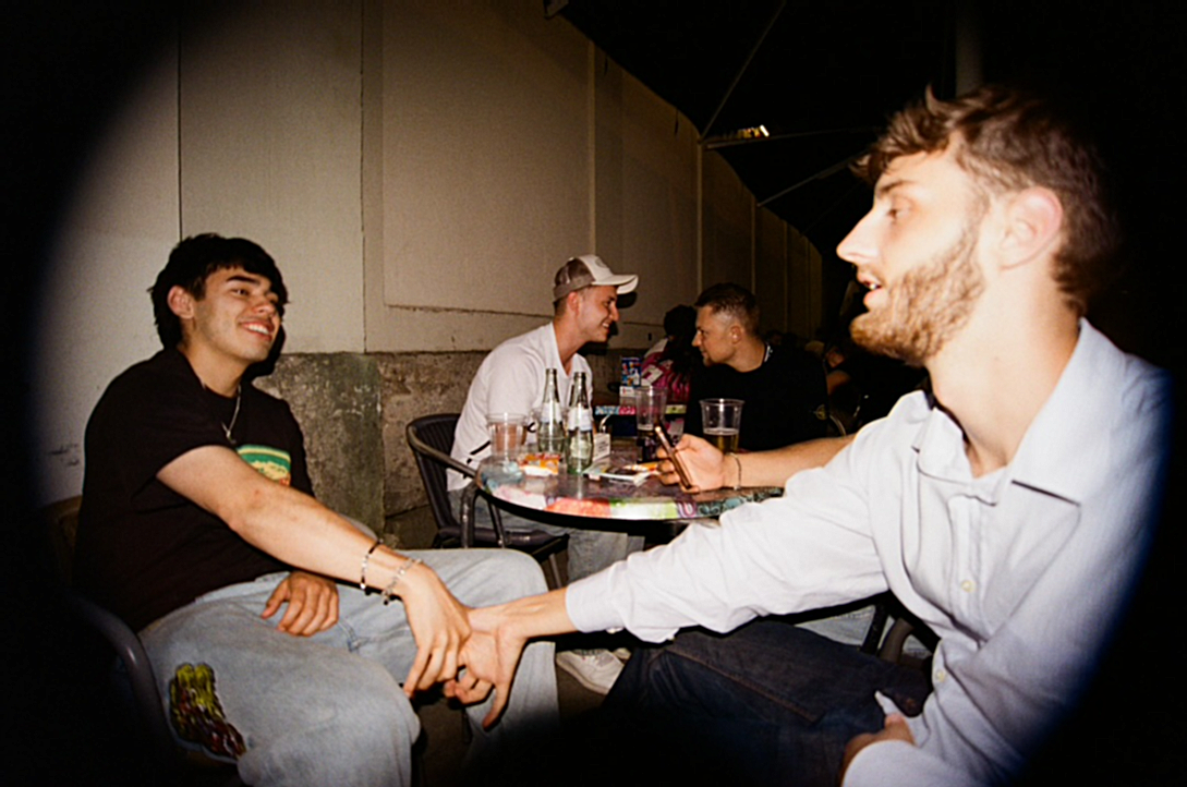
Left: Original, Center: Manually blurred input $(N=8, \sigma=1)$, Right: Sharpened blur ($factor=2.5$).
2.2 Hybrid Images
Next, I created hybrid images by combining high and low frequency components from different images. The idea comes from the fact that human visual perception is sensitive to high frequencies when viewing images up close, but primarily detects low frequencies when viewing from a distance. By blending different frequency ranges between two images, a single image can show different subjects depending on the distance it is viewed at.
The methodology works similarly to steps taken earlier. By applying a standard 2D Gaussian filter to extract low frequencies from one image, and creating a high-pass filter by subtracting the Gaussian-filtered version from the original image (equivalent to an impulse filter minus the Gaussian), we can overlay both outputs to produce the hybrid. Finding good cutoff frequencies (the $\sigma$ parameter for each Gaussian filter) requires some experimenting and really depends on the observer. For my implementation, I aligned image pairs using an alignment code (focussing on eye alignment for human subjects). Below is a rundown of the full process.

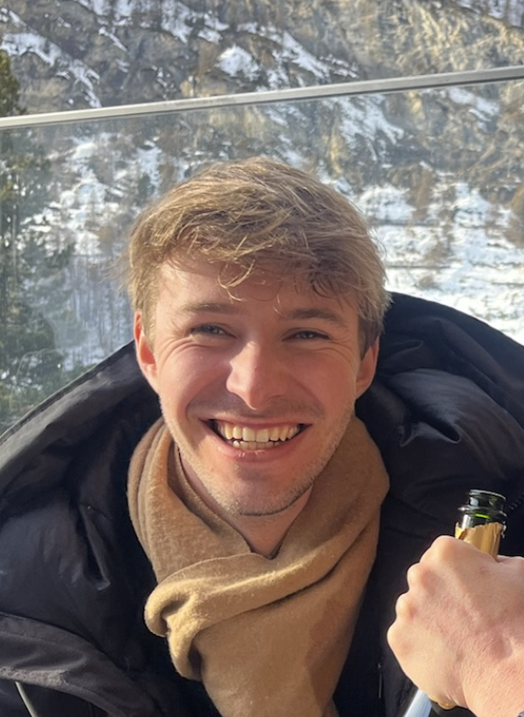
Left: Cyprian (high pass), unaligned, Right: Florentin (low pass), unaligned.
Then, I manually selected the alignment reference points on each image.


Left: Cyprian, aligned, Right: Florentin, aligned.
After some trial and error, I selected cutoff frequencies $\sigma_{low~pass} = 2.8,~\sigma_{high~pass} = 2.8$.
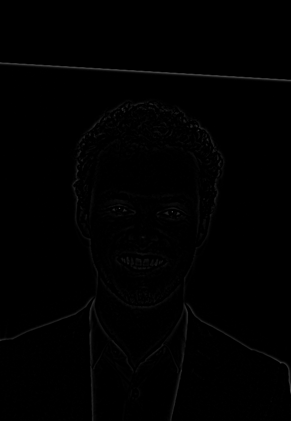
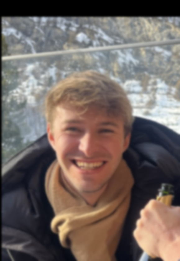
Left: Cyprian, high pass, Right: Florentin low pass.
Final overlayed output:
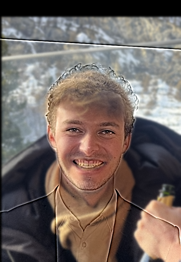
Cyprentin.
Fourier Transform Analysis
To get a better impression of how the hybrid image technique works, I analyzed the frequency content of each stage in the process. The Fourier transform visualizations show which spatial frequencies are present in each image. Low frequencies appear in the center, while high frequencies extend outward. This analysis reveals how our Gaussian and impulse filters isolate different frequency components.

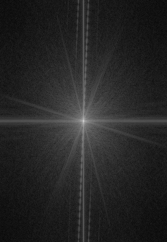
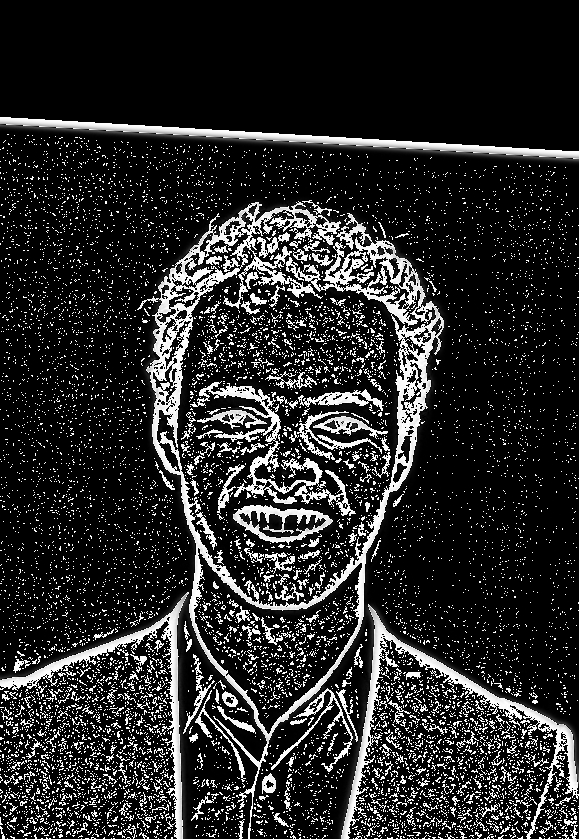
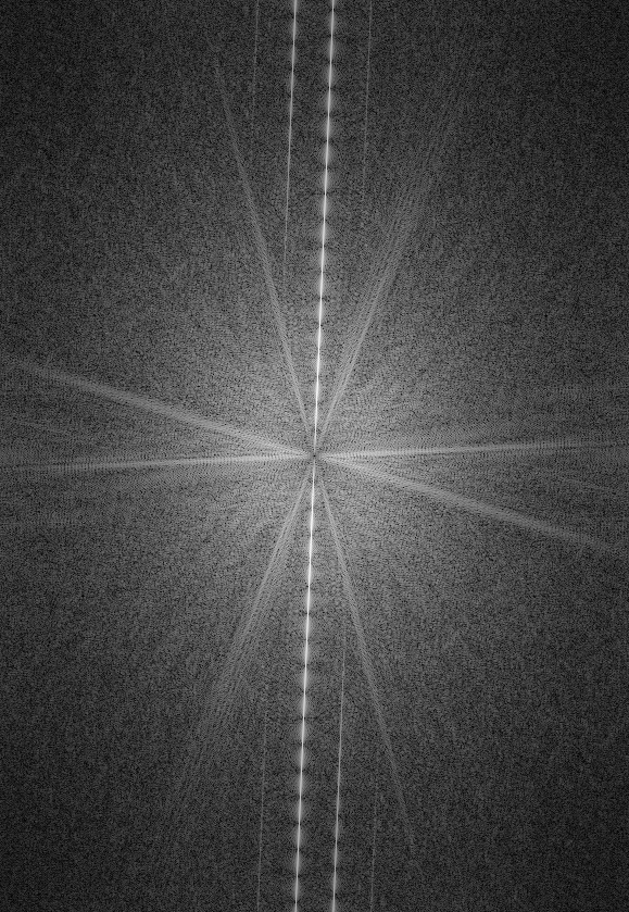
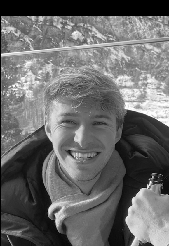
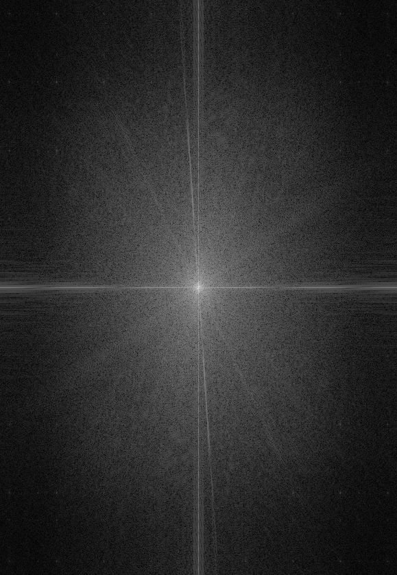

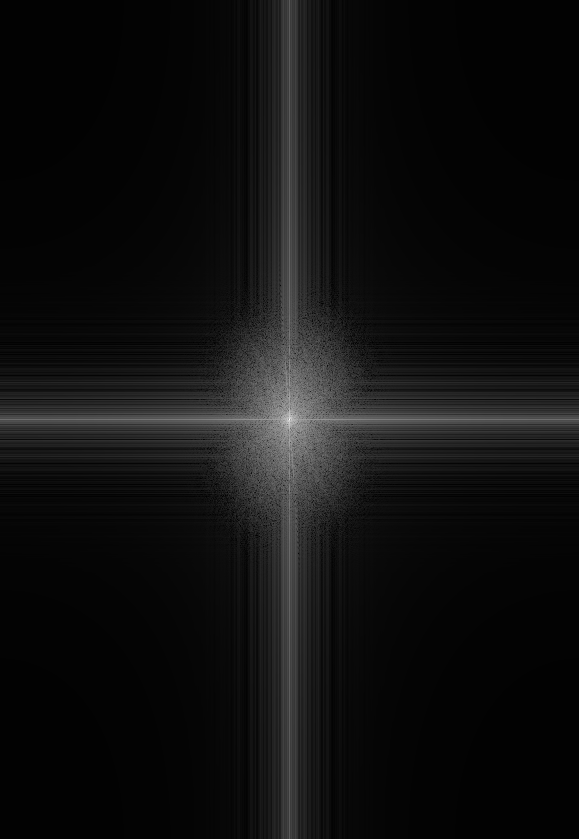
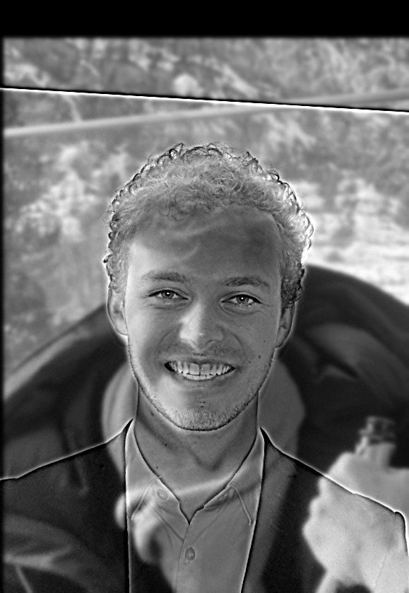
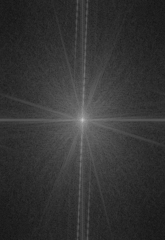
In the original images, the full spectrum of frequencies can be observed. When we apply the high-pass filter to Cyprian’s image, the FFT shows that low frequencies (near the center) are attenuated, leaving only the high-frequency edge information that defines facial features and fine details. Conversely, the low-pass filter applied to Florentin’s image preserves the central low frequencies while removing the high-frequency details. The combined hybrid image’s FFT shows how the two filtered images produce complementary frequency ranges.
Additional Examples
Below are more examples of hybrid images using the same methodology.
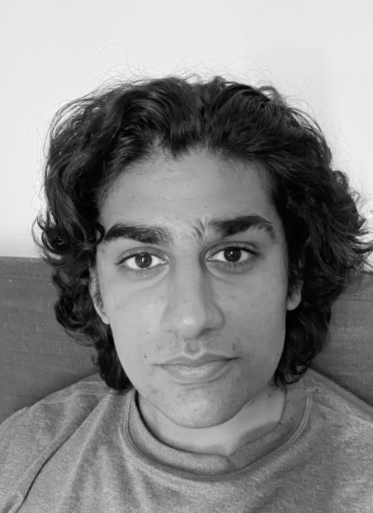

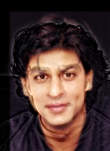
JJ and Khan hybrid: High frequencies from JJ, low frequencies from Khan ($\sigma_1=8, \sigma_2=2.5, \alpha=0.9$).
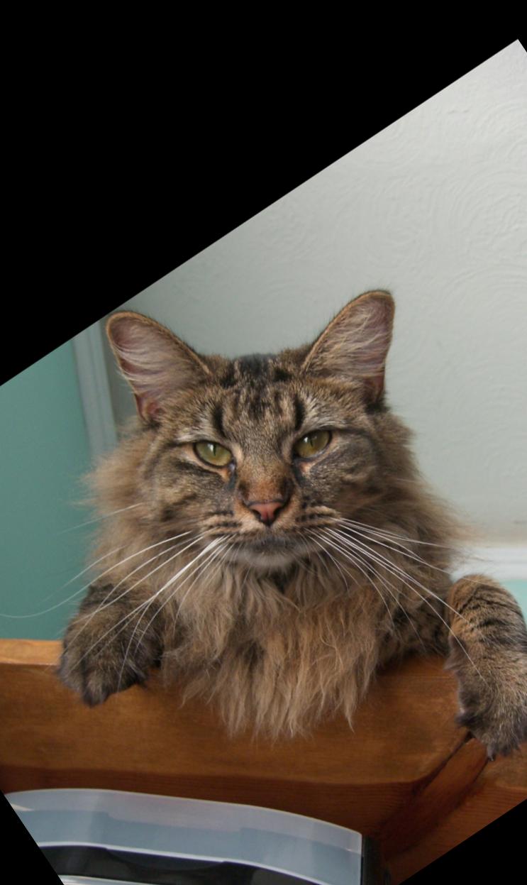
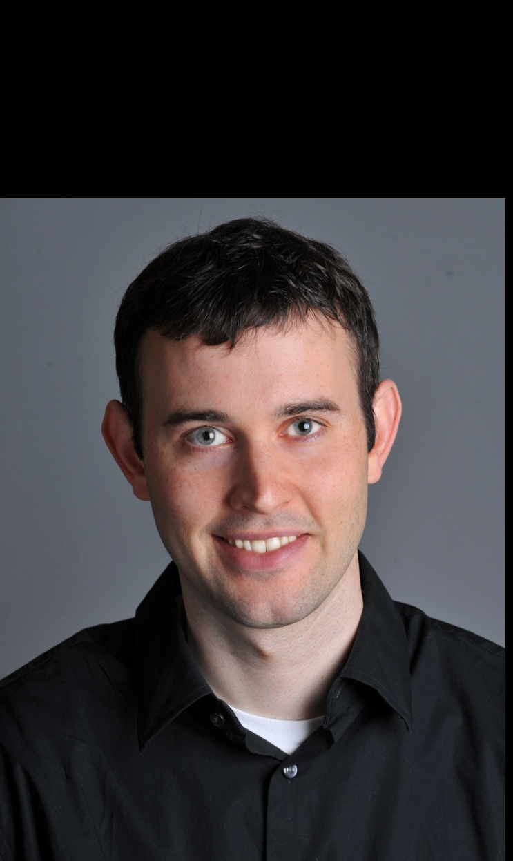
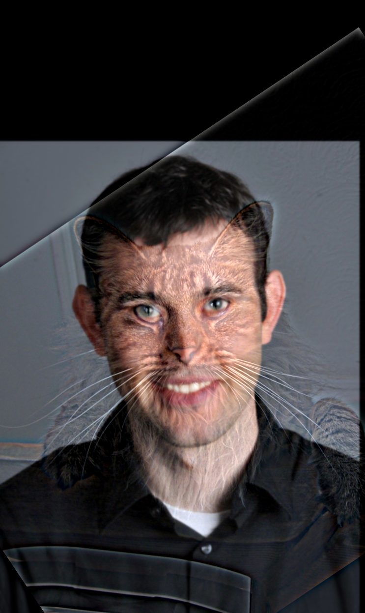
Nutmeg and Derek hybrid: High frequencies from cat (Nutmeg), low frequencies from Derek ($\sigma_1=8, \sigma_2=1.5, \alpha=0.9$).
2.3 Gaussian and Laplacian Stacks
In the next step of this project, I worked on blending two images seamlessly by applying a smoothed mask to lower frequencies and an unsmoothed mask to the highest frequencies. The effect of this approach is that coarser features, whose changes are easily noticeable to the eye, must be gradually blended, while finer features should be more aggressively blended to avoid perceiving blur artifacts. To accomplish this, I first isolated $N$ distinct frequency ranges for each of the two images being blended. This can be achieved by repeatedly applying Gaussian blur starting from each original image to form a Gaussian stack, then subtracting each $(i+1)$-th layer from the $i$-th layer to form a Laplacian stack. The last element in the Laplacian stack is simply the residual Gaussian blur. With these frequency decompositions, we can apply increasingly smoothed masks as we move toward coarser features.
Naive Apprach
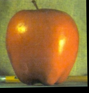
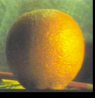
Reference images we want to blend.

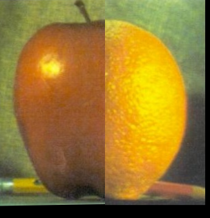
Left: Mask applied, Right: naive blend.
As we can see, simply “blending” both images by applying a uniform unsmoothed mask to both images produces an immediately identifiable stitch.
Gaussian Stack
Below is the Gaussian stack for both images, $N = 4$.


Level 0.


Level 1.

Level 2.

Level 3.
Laplacian Stack
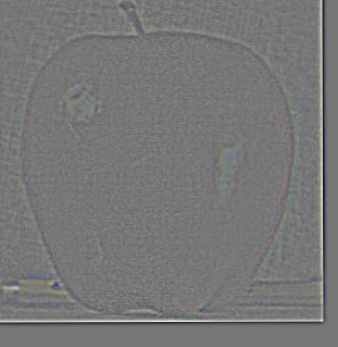
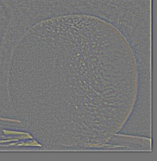
Level 0.
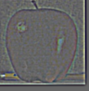
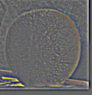
Level 1.
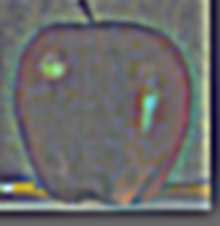
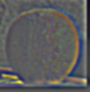
Level 2.


Level 3.
Now, onto multiresolution blending.
2.4 Multiresolution Blending
Applying the above vertical mask with increasing smoothing as we increase levels in the stack, we get the following level-by-level masked apples, oranges (using the inverse of the filter) and combined images.
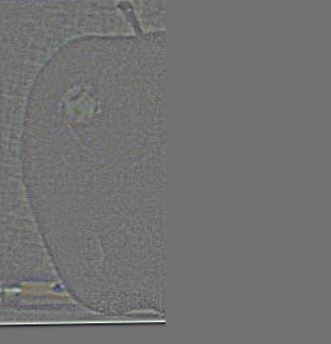
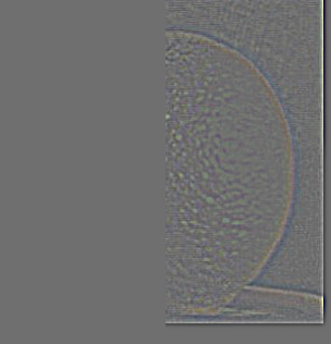
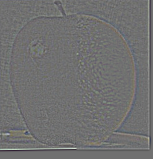
Level 0.
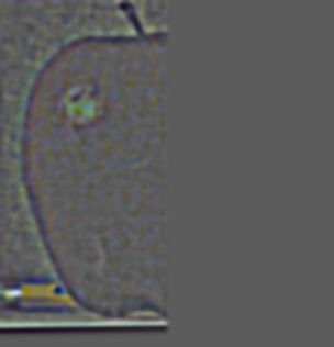
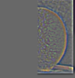
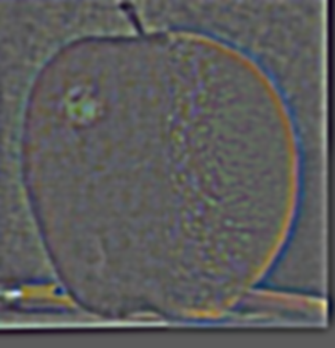
Level 1.
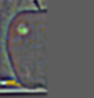
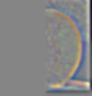
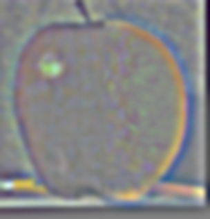
Level 2.

Level 3.
The key insight that makes multiresolution blending work at this stage is the additive property of Laplacian stacks. When we construct a Laplacian stack by computing differences between consecutive Gaussian levels, we create a frequency decomposition where each level contains a specific band of spatial frequencies. The crucial property is that the sum of all Laplacian levels perfectly reconstructs the original image.
If we have Gaussian levels $G_0, G_1, G_2, \ldots, G_N$ and Laplacian levels $L_0, L_1, L_2, \ldots, L_N$ where $L_i = G_i - G_{i+1}$ for $i = 0, 1, \ldots, N-1$ and $L_N = G_N$
Then $\sum_{i=0}^{N} L_i = L_0 + L_1 + L_2 + \cdots + L_N = G_0$
In short, we simply needed to add all layers of the stack together for the final blend:

The Oraple.
More Examples
Here are some more fun examples I developed.
Beach with mountains on the horizon

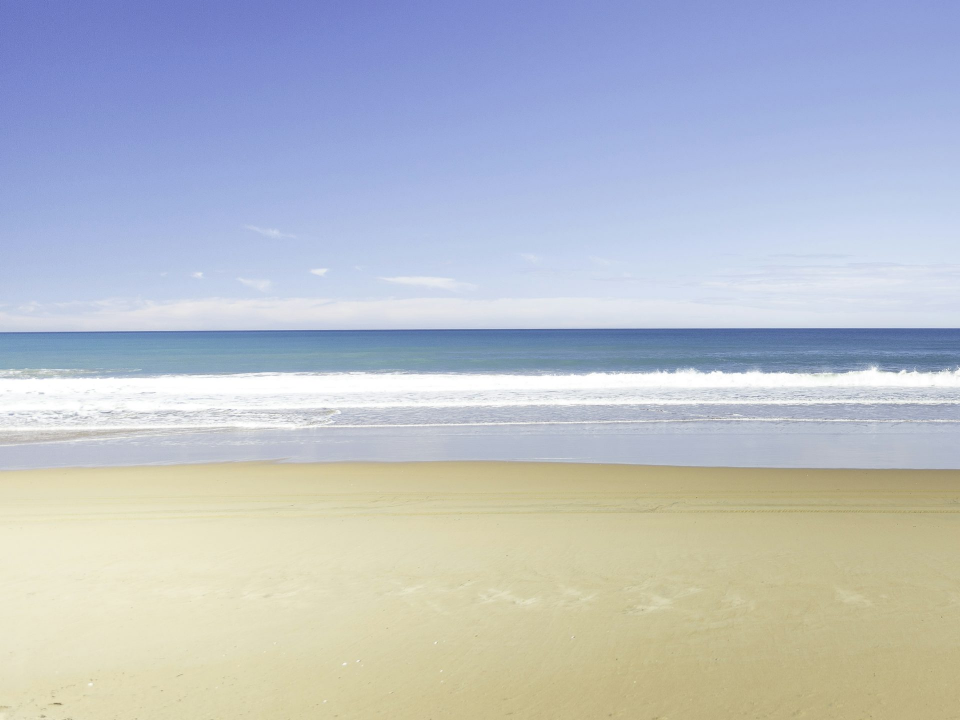

Left: Image 1, mountains, Center: Image 2, a beach, Right: Horizontal mask applied.
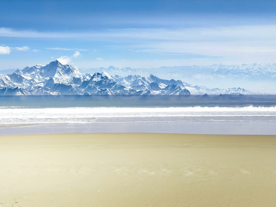
Beach with mountains on the horizon.
Interesting about this photo is how the coarse blend of the mountains looks like a shadow of the mountains on the water.
Electric bubble
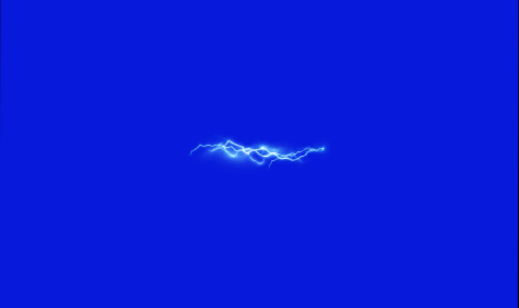
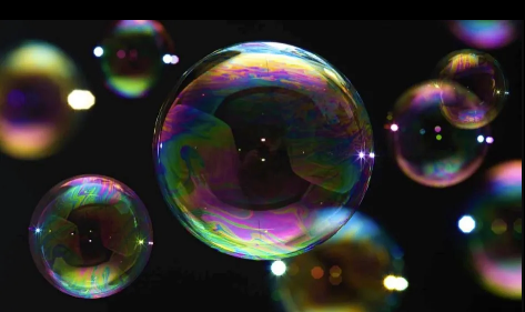
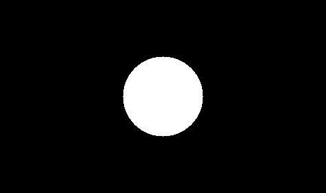
Left: Image 1, sparks, Center: Image 2, bubbles, Right: circular mask applied.
For this image, I wanted to create a slight variation of the blending approach, by only going for a 2-band blending and excluding the last Laplacian layer of the sparks image to remove the blue background.

Electric bubble.